
Here, we utilize a function called ‘Optimize,’ which instructs Amibroker to optimize the specified variable. The function’s signature is as follows:
optimize(“Description“, default, min, max, step);
where,
Description: Describes the parameter being optimized
Default: Default value to display if plotted on the chart
Min: Minimum value of the variable being optimized
Max: Maximum value of the variable being optimized
Step: Interval for increasing the value from min to max
Go to Analysis–>Optimize. Ensure your AFL file is selected in the Optimization window. The duration of this process may vary depending on the amount of historical data. Once the Optimization is completed, Amibroker will automatically display detailed results, sorted from best to worst. Here’s a snapshot of the Optimization result:
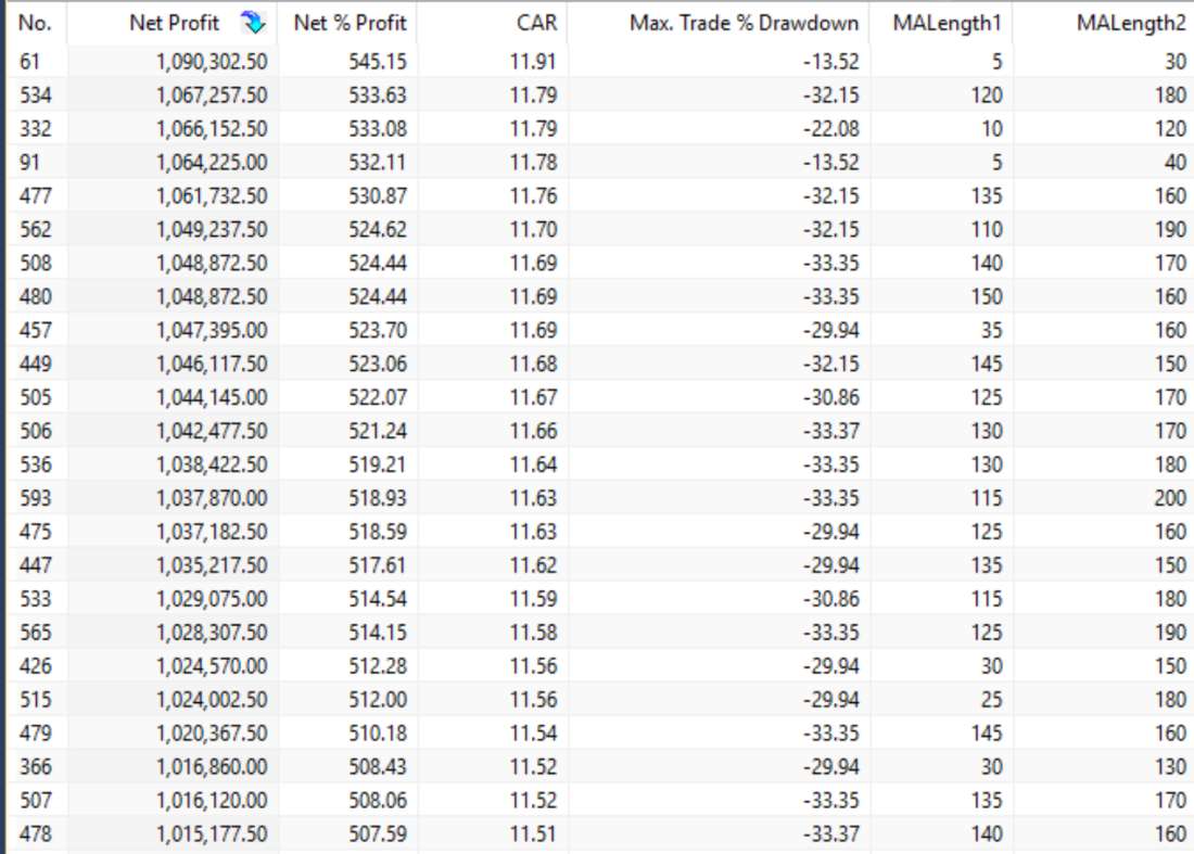
It’s evident that the combination of 5/30 EMA’s offers the best results with the least drawdown. Net profit has surged from 418% to 585%, and drawdown has dropped from 29% to 13%. You should test this same combination on different symbols and time frames to assess your Trading system’s robustness.
Step 5: Implementing Risk Management in Algorithmic Trading Systems
Constructing a successful Algorithmic Trading Systems with decent results is not sufficient. You must incorporate Risk Management to navigate unpredictable market risks. Explore our blog post that outlines detailed Risk Management strategies for Traders:
Mastering Risk Management: Strategies for Traders
You may have noticed that our simple Algorithmic system lacks a Stop Loss component. All long positions are closed based on the Sell signal. Let’s address this by adding a Stop Loss.
Insert the following line into your code:
ApplyStop is a Function that instructs Amibroker to exit the trade when predefined Stoploss or Target conditions are met. The function’s signature is as follows:
ApplyStop( type, mode, amount)
type =
0 = stopTypeLoss – maximum loss stop,
1 = stopTypeProfit – profit target stop,
2 = stopTypeTrailing – trailing stop,
3 = stopTypeNBar – N-bar stop
mode =
0 – disable stop (stopModeDisable),
1 – amount in percent (stopModePercent), or number of bars for N-bar stop (stopModeBars),
2 – amount in points (stopModePoint);
3 – amount in percent of profit (risk)
amount =
percent/point loss/profit trigger/risk amount.
This could be a number (static stop level) or an array (dynamic stop level)
Step 6: Monte Carlo Analysis
Monte Carlo simulation is a pivotal step in Trading system development and optimization. It involves repeatedly executing a predefined set of steps, introducing randomness to input parameters in each iteration. Results are recorded at the end of each iteration, forming the basis for probabilistic analysis. In Trading, Monte Carlo simulation is performed to forecast the success of a backtested trading system. To ensure that your trading system is robust, conduct multiple backtests with variations in your trading rules or data. If it consistently produces favorable results, it has a higher probability of generating profit. Learn more about performing Monte Carlo Analysis in Amibroker from the following post:
Mastering Monte Carlo Analysis in Amibroker Step by Step
Here’s a snapshot of the Monte Carlo Analysis report for our example Trading System:
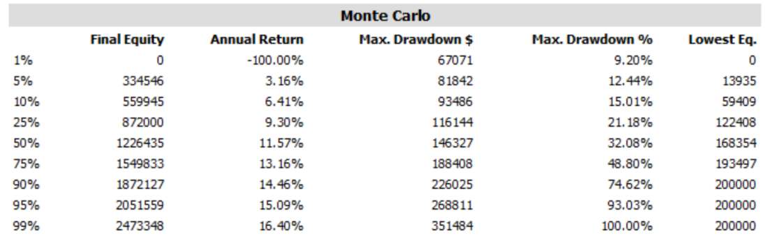
It is a well-established fact that ‘Markets are Random,’ and Monte Carlo simulation is a method to account for this randomness in your Trading system. If your system performs well in random market conditions, it has a significant probability of success. In the end, everything boils down to probability, which is the foundation of all profitable Trading systems. Relying solely on profitable backtest reports is insufficient. Monte Carlo analysis holds equal weight in system design.
Step 7: Automate Your Trading System
We strongly recommend trading manually for at least 6 months before considering full automation. Once you have confidence in your Trading System’s performance, start exploring automation.
Automatic or semi-automatic trading eliminates the impact of emotions on your trading decisions, as it directly executes orders in the terminal when your strategy generates signals. Many ready-made plugins and software are available in the market that can interpret buy/sell orders from Amibroker and place them in your Trading terminal. Check out the following post for a list of such software:
Top Auto Trading Software and Plugins in India
To fully automate your strategy, you will need a dealer terminal. Exchanges typically don’t allow fully automated platforms on retail terminals. To obtain a dealer terminal for NSE/BSE Segments, you will need to become an authorized person with your broker and pass the NISM-Series-VIII – Equity Derivatives Certification Examination. The procedure may vary for MCX. There will be a one-time cost to register as an Authorized person (you should check with your broker) and a rental fee for the dealer terminal, typically Rs 250 per segment per exchange.
So, you’ve developed your system, gained confidence in its performance, and possibly automated it. However, the story doesn’t end here. Markets are ever-changing, and so should your strategy. You need to regularly monitor your system’s performance and take note of anything that doesn’t align with your expectations. Always remember that you’ll never be able to devise a one-size-fits-all system that performs optimally in all market conditions.
Find the example AFL Trading system that we discussed throughout this article below: